Time Constant in An RLC Circuit

What’s Time Constant?

Time Constant (in physics and engineering), usually denoted by the Greek letter τ (tau), is the parameter characterizing the response to a step input of a first-order, linear time-invariant (LTI) system. The time constant is the main characteristic unit of a first-order LTI system.

In the time domain, the usual choice to explore the time response is through the step response to a step input, or the impulse response to a Dirac delta function input. In the frequency domain (for example, looking at the Fourier transform of the step response, or using an input that is a simple sinusoidal function of time) the time constant also determines the bandwidth of a first-order time-invariant system, that is, the frequency at which the output signal power drops to half the value it has at low frequencies.

The time constant is also used to characterize the frequency response of various signal processing systems – magnetic tapes, radio transmitters and receivers, record cutting and replay equipment, and digital filters – which can be modelled or approximated by first-order LTI systems. Other examples include time constant used in control systems for integral and derivative action controllers, which are often pneumatic, rather than electrical.

Time constants are a feature of the lumped system analysis (lumped capacity analysis method) for thermal systems, used when objects cool or warm uniformly under the influence of convective cooling or warming.

Physically, the time constant represents the elapsed time required for the system response to decay to zero if the system had continued to decay at the initial rate, because of the progressive change in the rate of decay the response will have actually decreased in value to 1 / e ≈ 36.8% in this time (say from a step decrease). In an increasing system, the time constant is the time for the system’s step response to reach 1 − 1 / e ≈ 63.2% of its final (asymptotic) value (say from a step increase). In radioactive decay the time constant is related to the decay constant (λ), and it represents both the mean lifetime of a decaying system (such as an atom) before it decays, or the time it takes for all but 36.8% of the atoms to decay. For this reason, the time constant is longer than the half-life, which is the time for only 50% of the atoms to decay.

Time Constant of an RLC Circuit

Reactive circuits are fundamental in real systems, ranging from power systems to RF circuits. They are also important for modeling the behavior of complex electrical circuits without well-defined geometry. An important part of understanding reactive circuits is to model them using the language of RLC circuits (An RLC circuit is an electrical circuit consisting of a resistor (R), an inductor (L), and a capacitor (C), connected in series or in parallel). The way in which simple RLC circuits are built and combined can produce complex electrical behavior that is useful for modeling electrical responses in more complex systems.

As all RLC circuits are second-order linear systems, they have some limit cycle in their transient behavior, which determines how they reach a steady state when driven between two different states. The time constant of an RLC circuit describes how a system transitions between two driving states in the time domain, and it’s a fundamental quantity used to describe more complex systems with resonances and transient behavior. If you’re working with RLC circuits, here’s how to determine the time constant in the transient response.

First-order and second-order systems (such as RL, RC, LC, or RLC circuits) can have some time constant that describes how long the circuit takes to transition between two states. Such a transition can occur when the driving source amplitude changes (e.g., a stepped voltage/current source) when the driving source changes frequency or when the driving source switches on or off. Because of this transition between two different driving states, it is natural to think of an RLC circuit in terms of its time constant.

In reality, an RLC circuit does not have a time constant in the same way as a charging capacitor. Instead, we say that the system has a damping constant which defines how the system transitions between two states. Because we are considering a second-order linear system (or coupled an equivalent first-order linear system) the system has two important quantities:

Damping constant (𝛽): This defines how energy initially given to the system is dissipated (normally as heat).
Natural frequency (𝜔₀): This defines how the system would oscillate if there were no damping in the system.

The time constant in an RLC circuit is basically equal to 𝛽, but the real transient response in these systems depends on the relationship between 𝛽 and 𝜔0. Second-order systems, like RLC circuits, are damped oscillators with well-defined limit cycles, so they exhibit damped oscillations in their transient response. The conditions for each type of transient response in a damped oscillator are summarized in the table below.

Condition	Type of Oscillation	Notes
𝜔₀ > 𝛽	Underdamped	The voltage/current exhibits an oscillation superimposed on top of an exponential rise.
𝜔₀ = 𝛽	Critically damped	The system will exhibit the fastest transition between two states without a superimposed oscillation.
𝜔₀ < 𝛽	Overdamped	The system does not exhibit any oscillation in its transient response. The transient response resembles that of a charging capacitor.

For simple underdamped RLC circuits, such as parallel or series RLC circuits, the damping constant can be determined by hand. Otherwise, such as in complex circuits with complex transfer functions, the time constant should be extracted from measurements or simulation data.

Extracting the Time Constant of an RLC Circuit from Measurements

If you have some measurements or simulation data from an RLC circuit, you can easily extract the time constant from an underdamped circuit using regression. Let’s look at a simple example for an underdamped RLC oscillator, followed by considerations for critically damped and overdamped RLC oscillators.

Underdamped

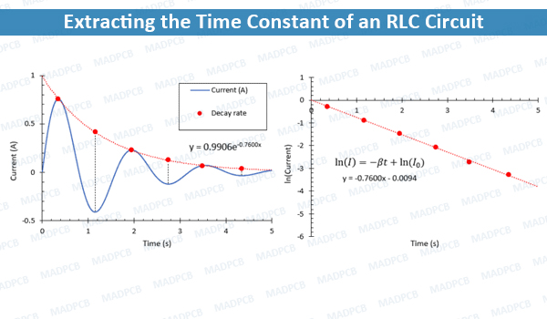
The graph below shows how this can easily be done for an underdamped oscillator. The data shows the total current in a series RLC circuit as a function of time, revealing a strongly underdamped oscillation. The successive maxima in the time-domain response (left) are marked with red dots. These data are then plotted on a natural log scale as a function of time and fit to a linear function. The slope of the linear function is 0.76, which is equal to the damping constant and the time constant. As a check, the same data in the linear plot (left panel) were fit to an exponential curve; we also find that the time constant in this exponential curve is 0.76.

Extracting the Time Constant of an RLC Circuit

In the above example, the time constant for the underdamped RLC circuit is equal to the damping constant. This is not the case for a critically damped or overdamped RLC circuit, and regression should be performed in these other two cases.

Critical Damping and Overdamping

In the case of critical damping, the time constant depends on the initial conditions in the system because one solution to the second-order system is a linear function of time. In an overdamped circuit, the time constant is no longer strictly equal to the damping constant. Instead, the time constant is equal to (Time constant of an overdamped RLC circuit):

τ = β±√(β-ω₀^2)

Here, we have a time constant that is derived from the sum of two decaying exponentials. When 𝜔0 << 𝛽, the time constant converges to 𝛽. The relationships discussed here are valid for simple RLC circuits with a single RLC block. More complex circuits need a different approach to extract transient behavior and damping.

Higher-Order RLC Circuits

Higher-order RLC circuits have multiple RLC blocks connected together in unique ways and they might not have a well-defined time constant that follows the simple equation shown above. While, in principle, you can calculate the response in the frequency domain by hand, circuits with a large number of RLC elements connected in a mix of series and parallel are very difficult to solve. The time constant you observe depends on several factors:

Where the circuit’s output ports are located.
How power sources and components are arranged into a larger topology.
Which voltage source is used for comparison in the circuit transfer function.

An example of a higher-order RLC circuit is shown below. In this circuit, we have multiple RLC blocks, each with its own damping constant and natural frequency.

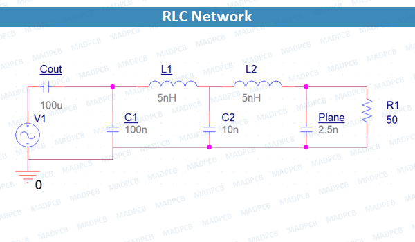
RLC Network

This is basically a higher-order filter, i.e., it mixes multiple filter sections together into a large RLC network. This type of circuit can have multiple resonances/anti-resonances at different frequencies and the frequencies may not be equal to the natural frequency of each RLC section. This occurs due to coupling between different sections in the circuit, producing a complex set of resonances/anti-resonances in the frequency domain.

There are two ways to determine the transient response and time constant of an RLC circuit from simulations:

Use a transient simulation, as was discussed above; simply fit the circuit’s time-domain response (natural log scale) and calculate the transfer function from the slope.
If you like determining transient responses by hand, you can use a frequency sweep to determine the poles and zeros in the transfer function.

Both methods can rely on using a powerful SPICE simulator to calculate the current and voltage seen at each component in the circuit. For complex circuits with multiple RLC blocks, pole-zero analysis is the fastest way to extract all information about the transient behavior, any resonant frequencies, and any anti-resonant frequencies.